
I have developed an interest in stochastic differential equations and have been studying them recently. However, I have found that the definition of integral used in these equations is different from the normal ones, such as Riemann Lebesgue integrals, and the complex calculations involved in solving even the simplest stochastic differential equation have been challenging for me. To overcome this difficulty, I decided to deepen my understanding of stochastic differential equations by simulating them. Since these equations describe the evolution of a function over a short time interval, simulating their behavior has been a relatively easy way for me to grasp the fundamental idea behind them. I have included the results of my simulations below, which I hope will be helpful for readers in understanding the basic concepts of stochastic differential equations.
Table of Contents
Black-Scholes Model
Black-Sholes model is a very fundamental model to describe option pricing. The equation is described below.
dS(t) = μS(t)dt + σS(t)dW(t)
where:
- W(t) is a standard Wiener process or Brownian motion.
- μ and σ are constant numbers.
The parameters μ and σ are commonly referred to as the drift rate and standard deviation of the underlying asset’s returns in the Black-Scholes model. However, as I am not very familiar with these concepts, I have simply defined them as constant numbers. Despite my limited understanding of these equations, I recognize that the main objective of the Black-Scholes model is to describe the movement of the underlying asset’s price over a short time interval. Therefore, to gain a better understanding of the model, I have attempted to simulate its behavior using the following equation.
S(t+Δt) = μS(t)*Δt + σS(t)*random() + S(t)
where:
- Δt is 1/10000.
- The number of trials is 10000.
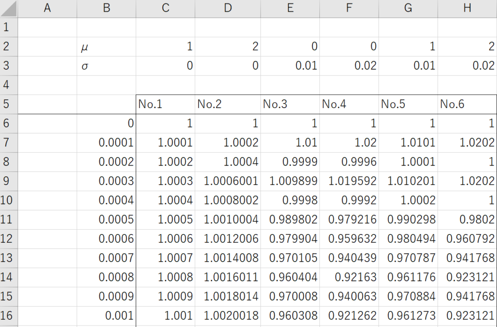
To make sure to understand the meaning of each item of the formula, I picked up some extreme examples as below.
- No.1: Set σ as 0 and μ as 1
- No.2: Set σ as 0 and μ as 2 (double the value of the No.1)
- No.3: Set μ as 0 and σ as 0.01
- No.4: Set μ as 0 and σ as 0.02 (double the value of the No.3)
- No.5: A combination of No.1 and No.3
- No.6: A combination of No.2 and No.4
First, I will present a comparison between No.1 and No.2. When σ is set to 0, the stochastic differential equation is equivalent to a differential equation whose solution is an exponential function. As a result, the graphs of the simulation are shown below.

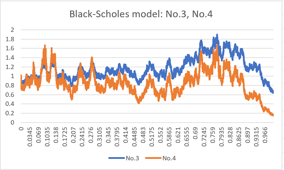
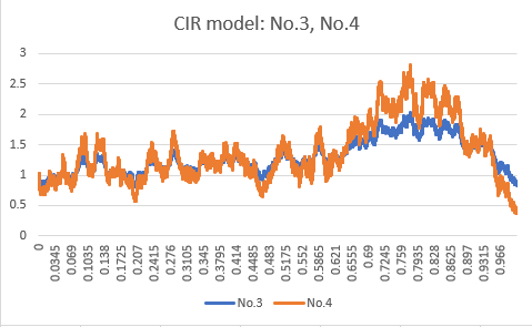
Next, I compared No.3 and No.4, where μ is set to 0. The second term of the Black-Scholes model is based on Brownian motion, which causes the trends to move randomly. However, the second term also includes the stochastic variable S(t), which means that the magnitude of volatility increases as S(t) becomes larger and decreases as S(t) becomes smaller. Unlike Brownian motion, I believe that this characteristic is the primary reason why the Black-Scholes model is utilized for option pricing.
Finally, I will present No.5 and No.6, which are combinations of No.1 and No.3, and No.2 and No.4, respectively. Compared to No.5, No.6 is attempting to increase due to the influence of μ, but ultimately decreases due to the regressive force of σ.

CIR Model
The CIR model is described by the following stochastic differential equation:
d r(t) = a (b – r(t)) dt + σ sqrt(r(t)) dW(t)
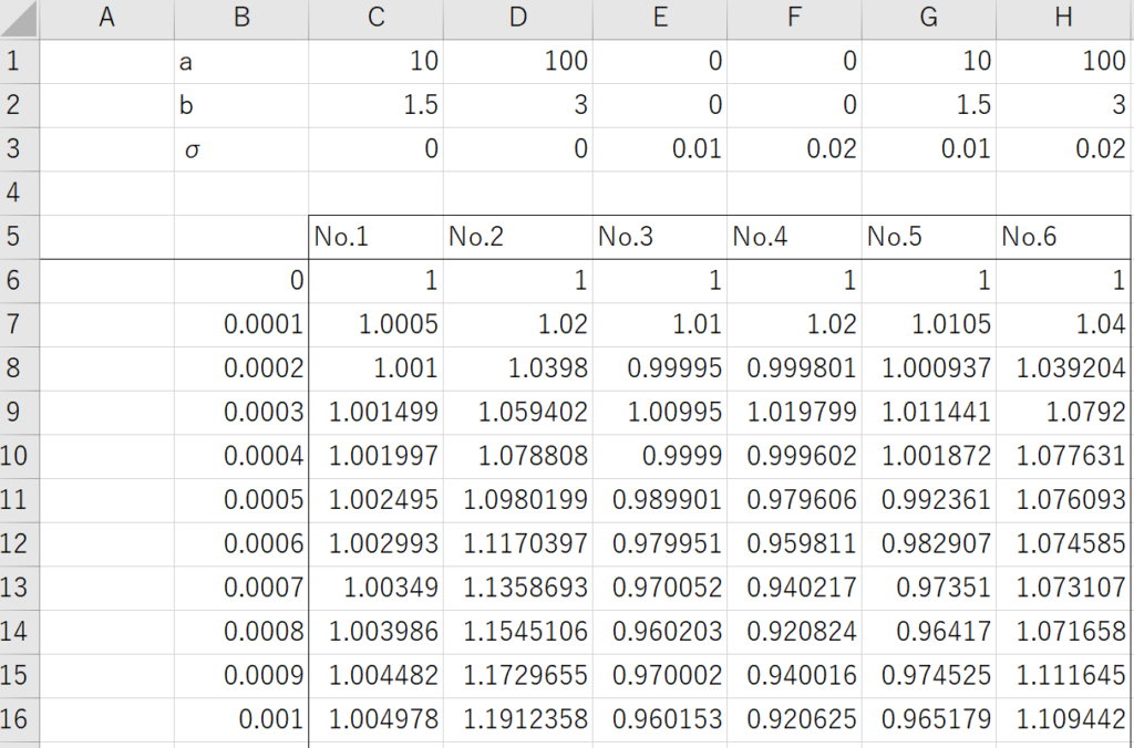
where dW(t) is a Wiener process (or Brownian motion) and a, b and σ are constant numbers. It is often described that r(t) is the interest rate at time t, a and b determine speed of mean reversion and the mean level, σ is the volatility parameter. Similar to the simulation of the Black-Scholes model that I showed above, I also pick up some examples as below.
- No.1: Set a as 10, b as 1.5 and σ as 0
- No.2: Set a as 100, b as 3 and σ as 0
- No.3: Set a as 0, b as 0 and σ as 0.01
- No.4: Set a as 0, b as 0 and σ as 0.02
- No.5: A combination of No.1 and No.3
- No.6: A combination of No.2 and No.4
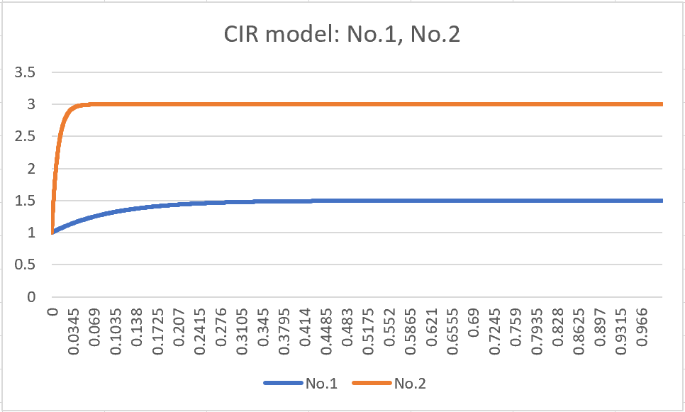
I will now present No.1 and No.2. From the graphs, we can observe that the parameter a determines the speed of the increase. It’s worth noting that the coefficient b – r(t) increases as r(t) becomes lower, and decreases as r(t) becomes higher. This causes it to converge to the parameter b.
The second term in the CIR model resembles the Black-Scholes model, with the magnitude of volatility increasing as r(t) becomes larger and decreasing as r(t) becomes smaller. However, the CIR model uses sqrt(r(t)) instead of r(t), resulting in a milder mean reversion trend as r(t) approaches 1, and a sharper trend as r(t) moves further away from 1.
The comparison between No.5 and No.6 describes below.
Two-Factor Gaussian Model
The two-factor Gaussian model can be described by the following system of stochastic differential equations.
dX(t) = – k1 X(t)dt + σ1 dW1(t)
dY(t) = – k2 Y(t)dt + σ2 dW2(t)
dW1(t) * dW2(t) = ρ dt
where X(t) and Y(t) are the two stochastic factors, W1(t) and W2(t) are two standard Brownian motions, k1 and k2 are the speed of mean reversion, and σ1 and σ2 are the volatilities of X(t) and Y(t), respectively. The two Brownian motions, W1(t) and W2(t), are assumed to be correlated with a correlation coefficient ρ, where -1 ≤ ρ ≤ 1.
Then, the short rate is given by
r(t) = x(t) + y(t)
I picked up the examples as below.
- No.1: Set k1 as 1, σ1 as 0.01 and assume r(t) = x(t)
- No.2: Set k1 as 100, σ1 as 0.02 and assume r(t) = x(t)
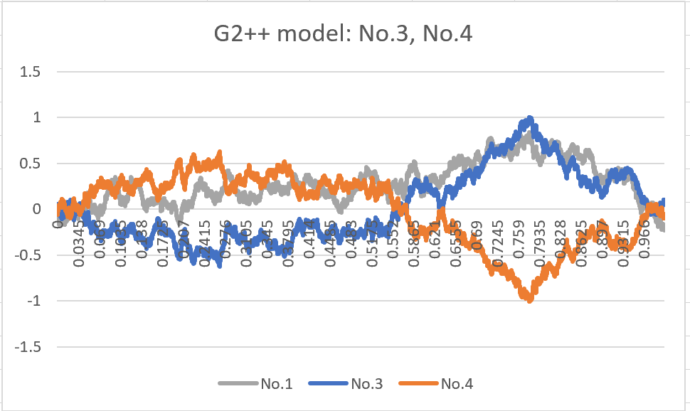
- No.3: Set k2 as 1, σ2 as 0.01, ρ as 0.5 and assume r(t) = y(t)
- No.4: Set k2 as 1, σ2 as 0.01, ρ as -0.5 and assume r(t) = y(t)
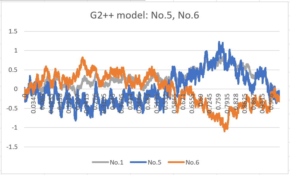
- No.5: Set k1 and k2 as 1, σ1 and σ2 as 0.01, ρ as 0.5 and assume r(t) = x(t) + y(t)
- No.6: Set k1 and k2 as 1, σ1 and σ2 as 0.01, ρ as -0.5 and assume r(t) = x(t) + y(t)
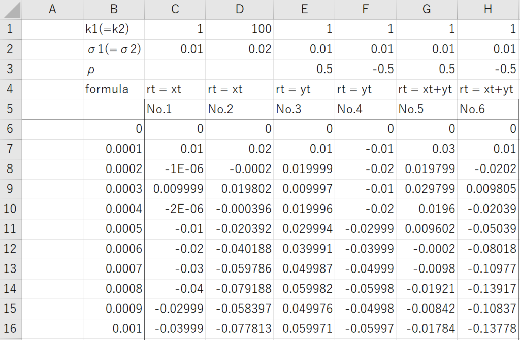
Firstly, I would like to explain the impact of the parameters k1(k2) and σ1(σ2). As shown in the table below, the mean reversion becomes more sensitive as the parameter k1(k2) increases, and the volatility increases as the parameter σ1(σ2) increases. These characteristics are similar to those observed in the previous models.
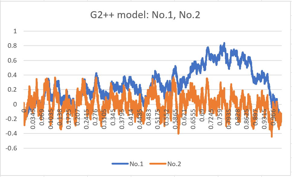
Next, I will present No.3 and No.4, which depict the trends under the assumptions of ρ = 0.5 and ρ = -0.5, respectively. As expected, the results align with my initial expectations.
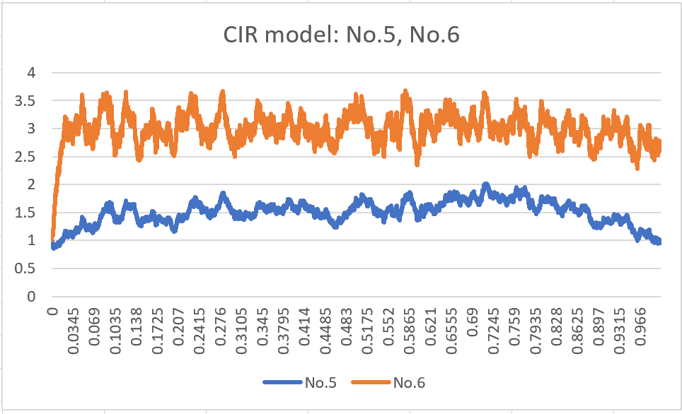
Finally, I will show the graphs of r(t) = x(t) + y(t).
Summary
Through basic examples of stochastic differential equations, I observed the impacts that each coefficient has on the results. In the Black-Scholes model, I understood that the trend increases due to the impact of the drift rate, while the force of mean reversion increases with standard deviation. In the CIR model, I observed that the trend moves around the mean level, and the speed of reaching the mean level is higher when the mean reversion is higher. In the Two-Factor Gaussian model, I observed how the two Brownian motions affect each other. As the next step, I would like to explore the pricing of derivatives and structured bonds.


Comments